1 November 2021 by Remco Bouckaert

Testing various hypotheses in a Bayesian setting is done through Bayes factors (the p-values of Bayesian statistics). There are many hypotheses that can be tested, for example

• whether the origin of clade falls within a certain time frame from time t0 to t1, or from time t2 to t3
• whether the root of a tree originates in a certain geographical region A or region B
• whether a strict clock is supported by the data or a relaxed clock
• whether a species assignment of lineages fits configuration A or configuration B (which allows species delimitation)
• whether substitution model X fits better than model Y or Z.

Note that we always formulate a hypothesis A together with another hypothesis B and we will estimate a Bayes factor that represents the evidence of “A versus B”, not “A versus not A”. So, it takes some care to formulate hypothesis of interest and specify them in a way that makes it a property that can be measured on the parameters and tree of a BEAST analysis.

Note: make sure the hypotheses matter.
If the question of interest is not changed by changing the hypothesis (e.g. strict vs
relaxed clock) there is no point in distinguishing the hypotheses.

Let us consider the following hypotheses on the origin of Indo-European languages:

• hypothesis A states it came from the steppen in the area from what is currently Ukraine spread by nomadic people around 5 to 6 thousand years ago, and
• hypothesis B states it originated in Anatolia in the current day Turkey through agriculture about 8 to 9 thousand years ago.

This translates into the following properties on a tree based on a large sample of Indo-European languages:

• hypothesis A: the root age is in the range 5-6kya
• hypothesis B: the root age is in the range 8-9kya

Note: this is just an example hypothesis, in this case on linguistic data.
Everything that follows is the same for hypotheses on nucleotide, amino acid, 
or other data.
Just keep in mind that you need to formulate 2 or more hypotheses

There are two main methods for estimating Bayes factors:

• estimate marginal likelihoods for hypothesis A and hypothesis B through path sampling, or nested sampling, and estimate Bayes factors from the marginal likelihoods, or
• measure the probabilities of the hypotheses being true in a prior sample and a posterior sample, and estimate Bayes factors from them.

The latter is more convenient, but is only possible if during the MCMC both hypotheses can become true. For the Indo-European sample, the tree can have a root in the range 5-6ky as in hypothesis A, and can move to the range 8-9kya as for hypothesis B. It is not always possible to jump between the hypotheses, for example, jumping between strict and relaxed clock is not implemented (yet), so requires running the more painful path or nested sampling route.

Bayes factors by path sampling/nested sampling

Only use path sampling or nested sampling if the MCMC does not allow both hypotheses to be available, because it takes less computational time and spares the effort of tuning and ensuring validity of the path sampling or nested sampling analyses. If that is not possible, proceed as follows:

• set up two BEAST XML files, where the hypothesis is enforced to be true. For the Indo-European example, this would mean setting a prior on the root age that restricts it to be in the range 5-6kya for hypothesis A, and 8-9kya for hypothesis B.
• run a path sampling or nested sampling analysis on each of the two XML files. Make sure these analyses are well tuned and valid by running performing multiple runs and other checks. If so, this provides us with two log marginal likelihood estimates, say ML(A) and ML(B).
• estimate the log Bayes factor as the difference of the two, so log(BF)=ML(A)-ML(B). If you want the actual Bayes factor, you can exponentiate this, but because differences between ML(A) and ML(B) can become quite large, be aware it is easy to end up with numerical problems.

See below on how to interpret the Bayes factor.

Bayes factors by sampling from prior and posterior

If the MCMC can move between the hypotheses, it is easier to sample from the prior and from the posterior and count how often the hypotheses occur in the prior and the posterior sample and calculate the Bayes factor from that. Note that it is not sufficient to only look at the posterior – if your prior favours one hypothesis greatly over the other, the posterior may reflect this as well, so just because the posterior favours one hypothesis over another that does not automatically mean that hypothesis is supported by the data/model in use.

To estimate the BF, proceed as follows:

• set of one BEAST XML file, and run it twice: one while sampling from the prior and one sampling from the posterior. You can sample from the prior by setting the -sampleFromPrior flag from the command line, set the attribute sampleFromPrior="true" in the XML, or check the sample from prior checkbox in the MCMC panel in BEAUti before saving the XML.
• count the number of times that hypothesis A is true and that hypothesis B is true for the prior run and for the posterior run. This may require a separate script, or you can manipulate the trace log in a spreadsheet: for the Indo-European origin example, loading the trace log in a spreadsheet, sorting the tree-height column, then checking how many entries are in the range 5-6kya and how many in 8-9kya may do the trick. So, now we have 4 counts: #A(prior), #A(post), #B(prior) and #B(post).
• estimate the Bayes factor as follows

     (#A(post)/#post)/(#A(prior)/#prior)
BF = -----------------------------------
     (#B(post)/#post)/(#B(prior)/#prior)

where #post=number of samples in posterior, and #prior=number of samples in prior. Instead of using maximum likelihood estimates, use Bayesian estimates aka Laplace correction by adding 1 observation for each hypothesis. And since #post and #prior cancels out, we get

     (#A(post)+1)/(#A(prior)+1)
BF = --------------------------
     (#B(post)+1)/(#B(prior)+1)

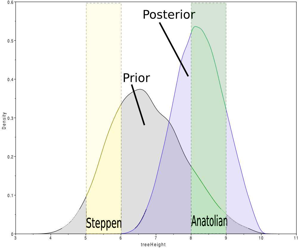
The graph above shows the prior and posterior distributions of the root age for Indo-European languages. The prior is chosen to be more or less symmetrically distributed over the two hypotheses (perhaps slightly preferring hypothesis 1). Note that there are quite a few samples where the prior is in between 6 and 8kya, which is an area not covered by any of the two hypotheses. This is to show that it is not necessary for the MCMC to be only in states that are hypothesised.

Root height has a prior mean of 6.8kya [4.9–8.8kya 95% HPD] while the posterior mean is 8.2kya [6.9 – 9.6kya 95% HPD] with almost no coverage of the 4-5kya range. In a trace log with 10.000 samples, taking off 10% burn-in, we have #prior = 90.000 = #posterior. In the prior, 1704 times the root age was in the 4-5kya range and 1498 times in the 8-9kya range. In the posterior, thes numbers were 16 and 4103 times respectively. Filling in the numbers in the first BF formula above, we get

BF = (16/1704)/(4103/1498) = 0.0034

Since the BF « 1, this shows there is more support for hypothesis 2 than or 1, so if we switch the hypotheses, and calculate the support for hypothesis 2 we get

BF = (4103/1498)/(16/1704) = 291.7

which is much larger than 100, indicating decisive support for hypothesis 2. Even when using the Laplace correction, the BF = ((4103+1)/(1498+1))/((16+1)/(1704+1)) = 274.6 » 100. See below on how to interpret the Bayes factor.

More than 2 hypotheses

When you have more than 2 hypotheses, you can

• pick a main hypothesis, e.g the most established hypothesis, and report all Bayes factors of all other hypotheses with respect to the main hypothesis, or
• if no hypothesis stands out from the rest of being the most established one, estimate Bayes factors comparing each of the hypothese pairwise.

Interpreting Bayes factors

The strength of support from Bayes factor (BF) comparisons of competing models can be evaluated using the framework of Kass & Raftery 1995.

A BF > 1 indicates support for hypothesis A, while a BF < 1 indicates support for hypothesis B. If the BF < 1, you can swap the hypotheses A and B to get a BF > 1. Kass & Raftery 1995 suggest the following interpretation:

• 1 < BF < 3.2 is not worth more than a bare mention,
• 3.2 < BF < 10 is substantial evidence,
• 10 < BF < 100 is strong support, and
• BF > 100 is decisive.

Note: Be aware when reading papers, which Bayes factor is reported
some times the log(BF) is multiplied by 2
some times the log(BF) is denoted as Bayes factor, leaving out the log
some times the raw Bayes factor is reported, i.e. exp(log(BF))
some time log based 2, or based 10 is used instead of the natural log

References

Kass RE, Raftery AE. Bayes factors. Journal of the American statistical association. 1995 Jun 1;90(430):773-95.