1 June 2022 by Remco Bouckaert
The same paper that introduced the BICEPS tree prior also introduced the Yule skyline model. This model is a pure birth model using epochs that integrates out the birth rates for each of the epochs. It is useful when all tips are sampled at the same time (i.e. no tip dates used in BEAUti) and there is reason to believe that speciation rates differed through time. The Yule skyline gets its efficiency by
- using smart tree moves,
- integrating out population sizes under a gamma prior, and
- fixing group sizes.
A tutorial for using the BICEPS tree prior can be found here. Essentially, you need to install the BICEPS package. Once you load an alignment into the Standard template in BEAUti, you can select the priors tab and under tree prior select Yule skyline. By default, the rate of the gamma distribution over the birth rate is estimated and has a log-normal hyper prior. Here, we will have a closer look at setting up the tree prior and the options provided.
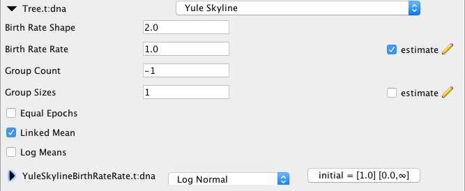
Birth Rate Shape
The shape of the gamma prior distribution on birth rates sizes is set to 2 by default. This provides a wide ranging distribution for population sizes. Increasing the value leads to linear increases in the variance.
Birth Rate Rate
Rate of the gamma prior distribution on birth rates. This parameterisation means the mean of the prior on birth rates is birth rate shape divided by birth rate rate.
When means are linked (Linked Mean checkbox is set), this only affects the first epoch (i.e. the one starting at the root). By default, the rate is estimated and comes with a log-normal distribution with mean of 1 in real space and variance of 1, which can be changed (see below), but does not seem to affect the inferred trees very much (see more below).
Group Count
Group count represents the number of groups used, which determines the dimension of the groupSizes parameter. If less than zero (default) 10 groups will be used, unless group sizes are larger than 30 (then group count = number of taxa/30) or less than 6 (then group count = number of taxa/6.
It can happen that because of the tendency to have fewer speciation events near the root of the tree per unit of time that the last group stretches over a relatively large amount of time. If group sizes are not estimated (the default behaviour) and group sizes are large this can lead to an unrealistic long episode of constant birth rate near the root of the tree. A solution to this problem is to use many small group sizes and link means.
Group Sizes
The group sizes parameter that determines the number of speciation events per group. If not estimated (estimate=false on this parameter), fixed group sizes will be used, otherwise they will be estimated.
Estimate group sizes?
In general, estimating group sizes is less efficient, since more parameters need to be used. On the other hand, it can be argued that assuming constant birth rates for a constant number of speciation events is not biologically plausible. However, by increasing the number of groups, the intervals at which birth rate is constant can be reduced so that the flexibility of estimated group sizes can be emulated while keeping group sizes constant but small (perhaps around 6).
When estimating group sizes it becomes necessary to interpret the trace file with some more care since ESSs displayed in Tracer may seem low while things are mixing fine. For example, consider the scenario where the data is produced by two groups of size G1 and G2 and constant (but substantially different) birth rates R1 and R2 between the groups. If we analyse this with 3 groups, we can capture this situation by using the first group size being G1 and the other two add up to G2. Alternatively, we can have the first two group sizes add up to G1, and G2 for the last group size. During the MCMC, it can happen on occasion that the state switches between these two states. This happens only occasionally, leading to low ESS values for group sizes as well as the birth rates, while there is no reason to be concerned about the analysis.
Initial group sizes?
The group sizes will be initialised automatically (as explained under the Group Count section above) when
- the group sizes entry has a different dimension (number of groups) than what is necessary based on the
group countvalue, or - the group size entries do not add up to the number of speciation events in the tree.
However, you can specify the group sizes by hand, for example for a tree with 50 taxa, which has 49 speciation events. If groupCount is set to 5, you can enter 15 10 10 10 4 in the group sizes entry and the group sizes will be fixed at these sizes. The group near the root will then only cover 4 speciation events while the youngest group covers 15 speciation events and all others 10.
Equal epochs option
If equalEpochs is false, use epochs based on groups from tree intervals, otherwise use equal sized epochs that scale with the tree height. If equalEpochs is set to true, the group sizes input is ignored.
Linked Mean
Use birth rate rate only for first epoch, and for other epochs use the posterior mean of the previous epoch. This makes the Yule skyline prior behave like a smoothing prior, which emulates the biologically plausible assumption that birth rates in consecutive epochs are related.
Log Means
Log mean population size estimates for each epoch. Apart from population sizes being logged based on the posterior population size for each epoch, this allows logging the mean of the posterior distribution. If set to true, two population size estimates appear in the log file.
Birth rate rate hyper prior
As mentioned above, the birth rate rate parameter is estimated by default, so that parameter requires a prior. By default, it is a log-normal distribution with mean of 1 (in real space) and variance of 1.
To test the sensitivity of the prior, we ran the HCV analysis example in the BICEPS repository with 63 taxa, 10 epochs, fixed group sizes and linked means. Below, you see a the estimates of first birth rate and all other birth size with different priors: mean of 0.1, 1, 10, 100, so 4 orders of magnitude difference between the lowest and highest mean value.

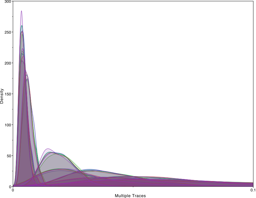
The last figure shows there seems to be very little impact on the birth rate estimates from the varying the rate. Zooming in on the first birth rate, which is supposed to be most sensitive to changes in the birth rate rate confirms there is not much sensitivity. The distribution of root height as well as reconstruction of speciation through time were similarly indistinguishable.
Of course, if you have prior information about a birth rates, do use it to set a good default value on the birth rate rate. Also, your data may differ, so check how different the posterior birth rate rate estimate is from the prior and if it differs substantially (orders of magnitude) make sure it does not impact your analysis by running with different priors and comparing the resulting trees and speciation rate reconstructions.
Yule skyline vs BICEPS
Both Yule skyline and BICEPS are flexible non-parametric tree priors. The Yule skyline is based on a pure birth process that is generally considered more appropriate when there are different species in the data, while the BICPS tree prior is based on the coalescent which assumes a well mixing population hence the data is from more closely related samples. However, since both priors allow a wide range of tree forms and shapes due to the epochs allowing changes through time in the tree generating process in both cases, both priors can be used if the parameters of the tree generating process are not of interest.
Below, a tree set comparison of the HVC data that compares BICPES trees with Yule skyline trees: they do not differ substantially.
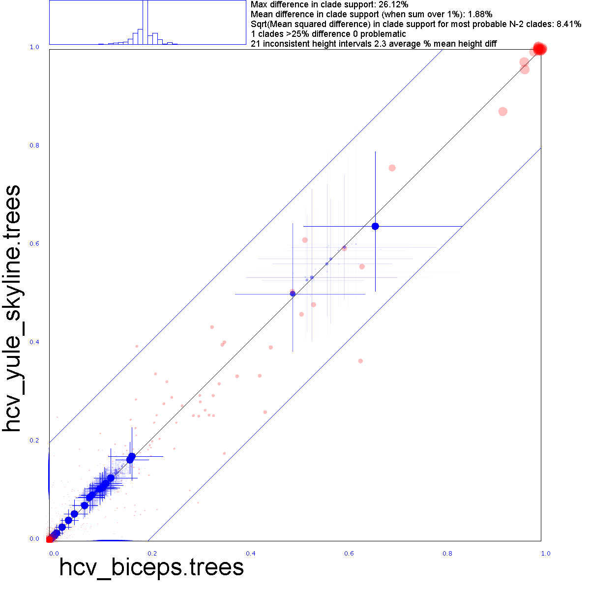
Red dots represent clade support, blue crosses clade heights and their 95% HPD intervals. More detail about the clade set comparison here.
Here are some considerations to choose between the two tree priors: Use Yule skyline if
- all tips are sampled at the same time, otherwise BICEPS is more appropriate
- more appropriate when data is from different species.
- you are interested in speciation rates through time.
- you are not interested in demographic reconstruction through time.
Use BICPES if
- one or more tips are sampled at different times.
- more appropriate when data is from closely related populations.
- you want to reconstruct population histories through time.
References
Remco R Bouckaert. An efficient coalescent epoch model for Bayesian phylogenetic inference. Sys Bio, syac015, 2022 doi:10.1093/sysbio/syac015