28 January 2019 by Sebastian Duchêne

In this post we discuss different approaches to assessing whether molecular sequence sampling times are sufficiently informative to calibrate the molecular clock, which is often done in studies of viruses, bacteria, and ancient DNA. Although there exist several methods for this purpose, they are difficult to interpret from a statistical standpoint and sometimes they require extensive computational resources. To address these limitations, we present a fully Bayesian alternative that should be easy to set up in BEAST2 and to interpret in empirical studies. As a proof of concept we use a small number of analyses, and in an upcoming study we investigate this approach in more detail.

Measurably evolving populations

Early molecular sequence studies of RNA viruses demonstrated that their genomes accumulate genetic change much more rapidly than other organisms. This has been attributed to the lack of repair mechanisms, short generation times, and selective constraints. A result of such rapid rates of evolution is that we can observe evolution in calendar time, such that samples collected a few months apart will exhibit a measurable amount of sequence divergence.

The molecular clock posits that evolutionary change occurs at an approximately constant rate over time (Zuckerkandl and Pauling 1965). Under this scenario molecular sequences of RNA viruses collected at different points in time will have a predictable amount of sequence divergence. In the context of phylogenetics, this means that we can use viral sequence sampling times to calibrate the molecular clock, instead of resorting to external sources of information, such as the fossil record. In a pioneering study, Korber et al. used HIV samples collected over a few years to calibrate the molecular clock and estimate the time of origin of some of the main human lineages (Korber et al. 2000). This approach has been extended to more sophisticated molecular clock models in many organisms (Rieux and Balloux 2016).

In 2003, Drummond et al. coined the term ‘measurably evolving populations’ for those organisms where the collection dates of the sequences span a sufficiently long time to produce an appreciable amount of genetic change (Drummond et al. 2003). In addition to RNA viruses, measurably evolving populations include DNA viruses and some bacteria. Moreover, the advent of ancient DNA from thousands or hundreds of thousands of years ago has meant that many molecular data sets of animals and plants can also be treated as measurably evolving.

Tests of temporal structure

In order to determine that a data set consists a measurably evolving population it is important to assess the temporal structure of the data. That is, whether the resulting inferences of evolutionary rates and times are informed by the sampling times. For example, if the collection times of the samples span a very short time, the timespan will not include a sufficient number of substitutions to estimate the evolutionary rate and timescale. In some viruses, such as influenza, obtaining samples over a few weeks might be sufficient, but in a mammalian data set it is typically necessary to use ancient DNA.

The most popular tests of temporal structure include the root-to-tip regression and the date-randomisation test. The root-to-tip regression consists in estimating a phylogenetic tree without a molecular clock (i.e., a phylogram) and conducting a regression of the distance from the root to each of the tips as a function of their collection times. The expectation is that samples that have been collected more recently should be more distant from the root of the tree. The slope of the regression corresponds to the evolutionary rate, the x-intercept is the time to the most recent common ancestor, and the R² measures the degree of clock-like behaviour. The root-to-tip regression provides a very valuable visual inspection of temporal structure, but it is not a formal statistical test (Rambaut et al. 2016).

The date-randomisation test consists in estimating the evolutionary rate using any phylogenetic method and repeating the analysis several times after randomising the sequence sampling times (Ramsden et al. 2008). The randomisation breaks the association of evolutionary distance and time, such that the resulting rate estimates represent the expectation of values if there were no temporal structure. The data are considered to have temporal structure if the rate estimate with the correct sampling times falls outside the range of values from the randomisations (Duchêne et al. 2015). Each randomisation is a complete separate analysis, such that the test requires substantial computation. One limitation of the date-randomisation test is that in some circumstances the test can fail to reject data sets with no temporal structure (Duchêne et al. 2015; Murray et al. 2015). The interpretation of the test has some similarities with frequentist hypothesis testing, which can lead to a mixture of Bayesian and frequentist approaches (when using Bayesian phylogenetic methods).

Bayesian assessment of temporal structure

In all Bayesian analyses, it is important to consider the prior carefully. Bayesian phylogenetic models sometimes involve a very large number of parameters, and it is a good idea to sample from the prior to verify that it is reasonable. This is easy to do in BEAUti by ticking the ‘Sample From Prior’ box at the bottom of the MCMC tab and it is equivalent to running the analysis without data (in practice, when selecting this option in BEAUti, BEAST2 will simply ignore the likelihood component of the xml file). Inspecting the prior is also useful to assess how informative the data are for inferences of interest. For example, if the prior on a given parameter is overly informative, then the posterior and prior may be identical, which means that the data are not providing any information beyond what was specified in the prior. Some parameters are non-identifiable, notably rates and times, such that the prior and posterior on calibrated internal nodes are usually expected to be identical (Warnock et al. 2012).

The intuition behind temporal structure is that there exists a strong association between the sequence data and their collection times. Consequently, for data with strong temporal structure the combination these two sources of information should result in a posterior distribution that is more informative than in the absence of temporal structure. Here we explore the prior and posterior distribution of the age of the root-node (tree height). We determine the informativeness of a distribution by calculating the 95% quantile width divided by the mean value, akin to measure of precision. Because we are interested in comparing the prior and posterior we obtain this measure for both, CV_prior and CV_posterior, respectively, and compute the ratio CV_ratio= CV_prior / CV_posterior. A CV_ratio that is higher than 1 means that the posterior is more informative than the prior.

We simulated sequence data using parameters inferred for H1N1 influenza, which typically has clock-like behaviour and strong temporal structure. The true evolutionary rate is 3.66×10-3 subs/site/year, the tree follows a coalescent process with exponential growth, the age of the root-node is 0.63 years, and the sampling times span half a year. We analyse the data using a matching model. The true phylogenetic tree is show in Fig 1. The prior and posterior for the age of the root-node are shown in Fig 2.

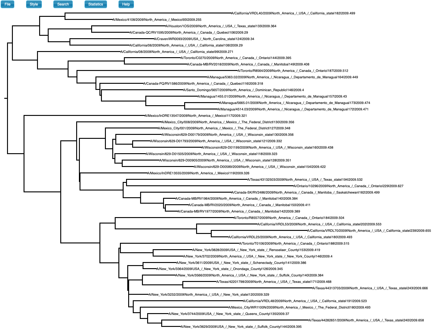
Fig 1. Phylogenetic tree of data set with temporal structure (generated in icytree.org).

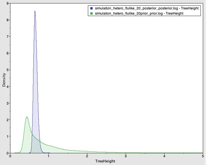
Fig 2. Prior and posterior densities (in green and blue, respectively) of the age of the root-node for a simulated data set with temporal structure.

The posterior 95% credible interval contains the value used to generate the data for the evolutionary rate (mean of 4.08×10-3 subs/site/year with credible interval of 2.5×10-3 to 5.9×10-3) and the age of the root-node (mean of 0.66 years with credible interval of 0.57 to 0.75). Importantly, the prior and posterior distributions largely overlap and the mean values are similar (at 0.66 for the posterior and 0.89 for the prior), but the prior is much more informative than the posterior, with a CV_ratio of 7.56.

We also simulate sequence data with no temporal structure (Fig 3). We use the same settings above, but the sampling times are all the same (i.e., the tree is ultrametric), such that there is no temporal structure. For the analysis, however, we set sampling times from a typical influenza data set and which span half a year. The prior and posterior distributions of the age of the root-node are shown in Fig 4. As expected, the posterior estimates of the evolutionary rate (mean of 6.83×10-4 subs/site year with credible interval of 2.30×10-4 to 1.25×10-3) and the age of the root-node do not include the values used to generate the data (mean of 2.09 with credible interval of 0.88 to 3.62). The CV_ratio is 1.6 and much lower than in the simulation with temporal structure.

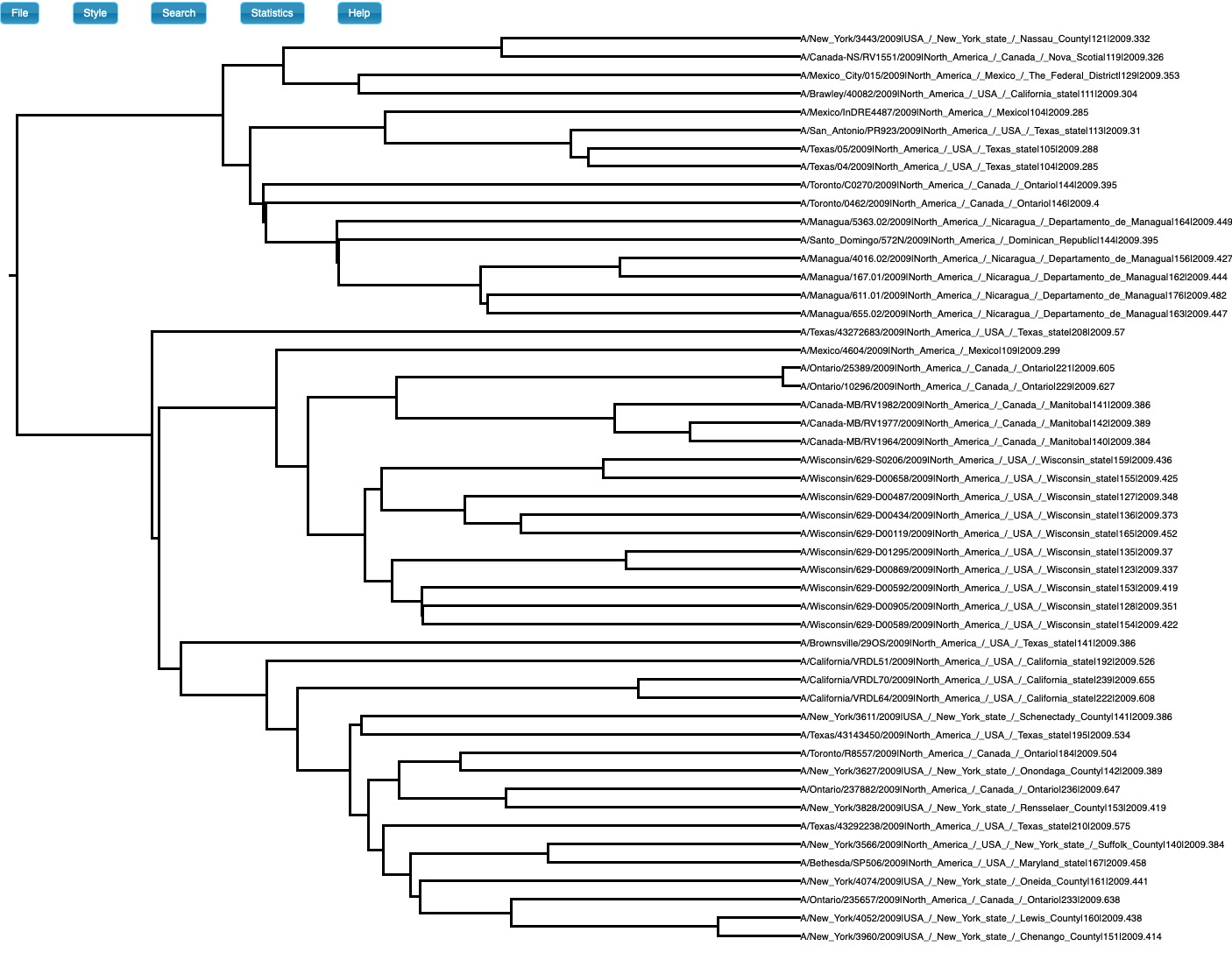
Fig 3. Phylogenetic tree of data set with no temporal structure (generated in icytree.org). Note that the tree is ultrametric, but the tip labels have sampling times which were used for the analyses in BEAST2.

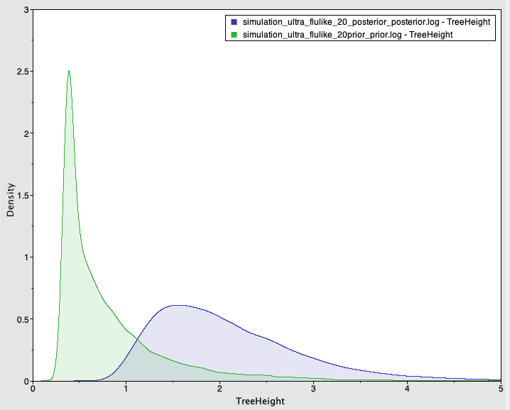
Fig 4. Prior and posterior densities (in green and blue, respectively) of the age of the root-node for a simulated data set with no temporal structure.

In the simulations with and without temporal structure the CV_ratio is higher than 1. Thus, to devise guidelines for the expected CV_ratio of the age of the root-node when there is temporal structure we generated 100 data sets with and without temporal structure and investigated the range of values of the CV_ratio in both scenarios. As shown in Fig 5, data sets with temporal structure have a CV_ratio of 5 or higher, whereas those with no temporal structure have values of at most 2.5. For empirical data analysed with similar settings as used here a CV_ratio of at least 5 is necessary to consider that there is temporal structure and that the estimates are reliable.

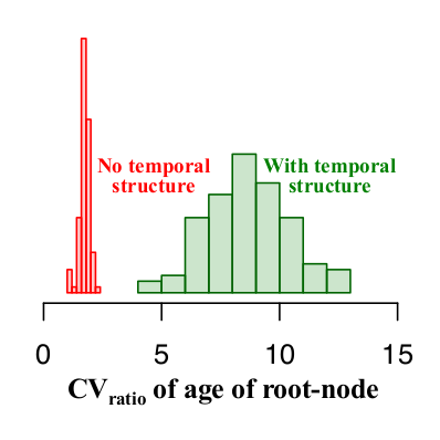
Fig 5. Histograms of the CV_ratio of the age of the root-node for 100 simulations with and without temporal structure (in green and red, respectively).

Conclusion

Comparing the prior and posterior distributions is a key aspect in Bayesian analyses. In principle, such comparisons are useful to verify that the marginal prior is sensible and that the data are informative. Here we illustrate an application specifically for assessing temporal structure which can be useful for analyses of rapidly evolving organisms or those that involve ancient DNA. The CV_ratio of the age of the root-node appears to be a useful measure for this purpose under a simple phylogenetic model, but it is important to note that tree priors generate different expectations of the ages of internal nodes. For instance, birth-death models that explicitly describe the sampling process have different prior expectations on the ages of internal nodes than coalescent models. For this reason, it is important to assess the prior carefully before interpreting any estimates.

Other parameters that may be useful for assessing temporal structure include the evolutionary rate. However, the prior on this parameter is often very vague (e.g., it has a uniform distribution between 0 and infinity as the default in BEAUti). In such circumstances, obtaining sufficient samples from the prior may very difficult or impossible. Even if sampling from the prior is possible, if it is very vague then even data with no temporal structure can produce a posterior that is much more informative than the prior. In an upcoming study we will investigate this and other theoretical aspects of Bayesian tests of temporal structure.

Finally, conducting these analyses in BEAST2 is simple. After setting up the complete model in BEAUti, create the xml file and give the file names the ‘_posterior’ extension (e.g., myanalysis_posterior.xml, myanalysis_posterior.log, myanalysis_posterior.trees). Then in the MCMC tab tick the box ‘Sample From Prior’ and save the files with the extension ‘_prior’ (e.g., myanalysis_prior.xml, myanalysis_prior.log, myanalysis_prior.trees). To compare the prior and posterior load the _posterior.log and _prior.log files in Tracer. The CV_ratio can be calculated by taking the 95% HPD and mean values of the ‘TreeHeight’ trace.

References

• Drummond A.J., Pybus O.G., Rambaut A., Forsberg R., Rodrigo A.G. 2003. Measurably evolving populations. Trends Ecol. Evol. 18:481–488.
• Duchêne S., Duchêne D., Holmes E.C., Ho S.Y.W. 2015. The performance of the date-randomisation test in phylogenetic analyses of time-structured virus data. Mol. Biol. Evol. 32:1895-1906.
• Korber B., Muldoon M., Theiler J., Gao F., Gupta R., Lapedes A., Hahn B.H., Wolinsky S., Bhattacharya T. 2000. Timing the ancestor of the HIV-1 pandemic strains. Science. 288:1789–1796.
• Murray G.G.R., Wang F., Harrison E.M., Paterson G.K., Mather A.E., Harris S.R., Holmes M.A., Rambaut A., Welch J.J. 2015. The effect of genetic structure on molecular dating and tests for temporal signal. Methods Ecol. Evol. 7:80–89.
• Rambaut A., Lam T.T., Carvalho L.M., Pybus O.G. 2016. Exploring the temporal structure of heterochronous sequences using TempEst (formerly Path-O-Gen). Virus Evol. 2:vew007.
• Ramsden C., Melo F.L.L., Figueiredo L.M.M., Holmes E.C.C., Zanotto P.M.A.M.A. 2008. High rates of molecular evolution in hantaviruses. Mol. Biol. Evol. 25:1488–1492.
• Rieux A., Balloux F. 2016. Inferences from tip-calibrated phylogenies: a review and a practical guide. Mol. Ecol. 25:1911–1924.
• Warnock R.C.M., Yang Z., Donoghue P.C.J. 2012. Exploring uncertainty in the calibration of the molecular clock. Biol. Lett. 8:156–159.
• Zuckerkandl E., Pauling L. 1965. Evolutionary divergence and convergence in proteins. In: Bryson V., Vogel H., editors. Evolving Genes and Proteins. New York: Academic press. p. 97–166.