1 May 2022 by Remco Bouckaert

Recently, we presented a two headed approach called Bayesian Integrated Coalescent Epoch PlotS (BICEPS) for efficient inference of coalescent epoch models. The BICEPS tree prior can be considered a more muscular version of the popular Bayesian skyline model. It divides time in groups and assumes a piecewise linear population function. BICEPS gets its efficiency by

• using smart tree moves,
• integrating out population sizes under an inverse gamma prior, and
• fixing group sizes.

A tutorial for using the BICEPS tree prior can be found here. You need to install the BICEPS package. Once you load an alignment into the Standard template in BEAUti, you can select the priors tab and under tree prior select BICEPS. By default, the population mean is estimated and has a log-normal hyper prior. Here, we will have a closer look at setting up the tree prior and the options provided.

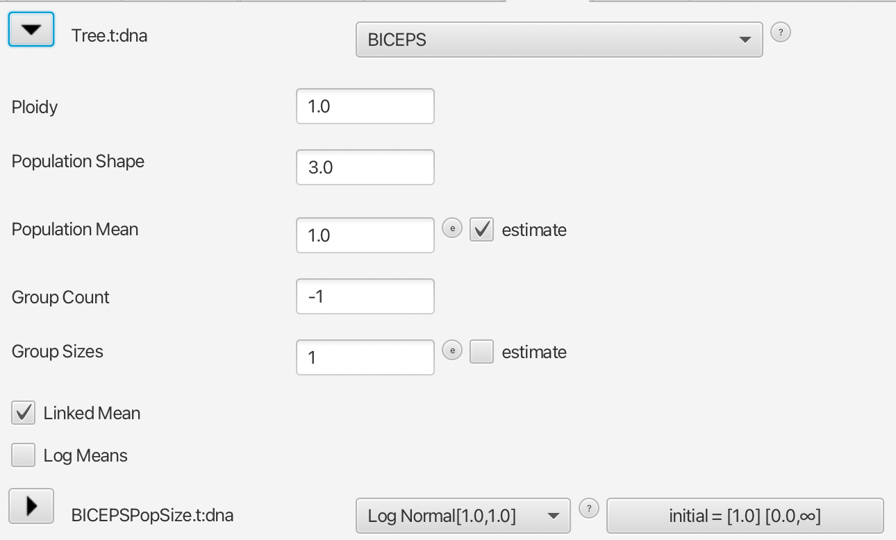
Ploidy

Ploidy (copy number) for the gene, typically a whole number or half (default is 1) autosomal nuclear: 2, X: 1.5, Y: 0.5, most viral: 1, mitrochondrial: 0.5. Using the wrong ploidy results in population sizes being estimated incorrectly, and only affects estimate of the tree through the prior on population mean (which we will later see BICEPS seems quite insensitive to).

Population Shape

The shape of the inverse gamma prior distribution on population sizes is set to 3 by default, which makes the coefficient of variation of the distribution being 1. This provides a wide ranging distribution for population sizes. Increasing the value leads to lower variance.

Population Mean

Mean of the inverse gamma prior distribution on population sizes. When means are linked, this only affects the first epoch (i.e. the one starting at the most recent tip). By default, the mean is estimated and comes with a log-normal distribution with mean of 1 in real space and variance of 1, which can be changed (see below), but does not seem to affect the inferred trees very much (see more below).

Group Count

Group count represents the number of groups used, which determines the dimension of the groupSizes parameter. If less than zero (default) 10 groups will be used, unless group sizes are larger than 30 (then group count = number of taxa/30) or less than 6 (then group count = number of taxa/6.

It can happen that because of the tendency to have fewer coalescent events near the root of the tree per unit of time that the last group stretches over a relatively large amount of time. If group sizes are not estimated (the default behaviour) and group sizes are large this can lead to an unrealistic long episode of constant population size near the root of the tree. A solution to this problem is to use many small group sizes and link means.

Group Sizes

The group sizes parameter that determines the number of coalescent events per group. If not estimated (estimate=false on this parameter), fixed group sizes will be used, otherwise they will be estimated.

Estimate group sizes?

In general, estimating group sizes is less efficient, since more parameters need to be used. On the other hand, it can be argued that assuming constant population sizes for a constant number of coalescent events is not biologically plausible. However, by increasing the number of groups, the intervals at which population size is constant can be reduced so that the flexibility of estimated group sizes can be emulated while keeping group sizes constant but small (perhaps around 6).

When estimating group sizes it becomes necessary to interpret the trace file with some more care since ESSs displayed in Tracer may seem low while things are mixing fine. For example, consider the scenario where the data is produced by two groups of size G1 and G2 and constant (but substantially different) population sizes N1 and N2 between the groups. If we analyse this with 3 groups, we can capture this situation by using the first group size being G1 and the other two add up to G2. Alternatively, we can have the first two group sizes add up to G1, and G2 for the last group size. During the MCMC, it can happen on occasion that the state switches between these two states. This happens only occasionally, leading to low ESS values for group sizes as well as the population sizes, while there is no reason to be concerned about the analysis.

Initial group sizes?

The group sizes will be initialised automatically (as explained under the Group Count section above) when

• the group sizes entry has a different dimension (number of groups) than what is necessary based on the group count value, or
• the group size entries do not add up to the number of coalescent events in the tree.

However, you can specify the group sizes by hand, for example for a tree with 50 taxa, which has 49 coalescent events. If groupCount is set to 5, you can enter 15 10 10 10 4 in the group sizes entry and the group sizes will be fixed at these sizes. The group near the root will then only cover 4 coalescent events while the youngest group covers 15 coalescent events and all others 10.

Linked Mean

Use populationMean only for first epoch, and for other epochs use the posterior mean of the previous epoch. This makes BICEPS behave like a smoothing prior, which emulates the biologically plausible assumption that population sizes in consecutive epochs are related. When means are not linked, especially when group sizes are small, this may lead to wild variation of population sizes in consecutive epochs, and clumping of nodes in epochs with very small population sizes.

Log Means

Log mean population size estimates for each epoch. Apart from population sizes being logged based on the posterior population size for each epoch, this allows logging the mean of the posterior distribution. If set to true, two population size estimates appear in the log file.

Population Mean hyper prior

As mentioned above, the mean population size parameter is estimated by default, so that parameter requires a prior. By default, it is a log-normal distribution with mean of 1 (in real space) and variance of 1.

Below, you see a the estimates of first population size and second population size with different priors: mean of 0.1, 1, 10, 100, so 4 orders of magnitude difference between the lowest and highest mean value. This is a covid analysis with 257 taxa, 10 epochs, fixed group sizes and linked population means.

As you can see, there is a small effect on the first population size estimate, where the modes are in order of the size of the population size priors. The second population size estimates are indistinguishable, so after 26 coalescent events the prior appears to have been drowned out by the data, suggesting a small sensitivity to the population size prior. The following 8 group size estimates are equally similar. Unsurprisingly, demographic reconstructions under these four priors were indistinguishable as well.

Of course, if you have prior information about a population size, do use it. Also, your data may differ, so check how different the posterior mean population estimate is from the prior and if it differs substantially (orders of magnitude) make sure it does not impact your analysis by running with different priors and comparing the resulting trees and demographic reconstructions.

Equal epochs option

This option is not shown in BEAUti, since it is not particularly well tested. If equalEpochs is false, use epochs based on groups from tree intervals, otherwise use equal sized epochs that scale with the tree height. If true, the group sizes input is ignored. If you want to use it, you need to edit the XML in a text editor and set the equalEpochs attribute to true on the distribution element containing BICEPS.

References

Remco R Bouckaert. An efficient coalescent epoch model for Bayesian phylogenetic inference. Sys Bio, syac015, 2022 doi:10.1093/sysbio/syac015