1 February 2025 by Remco Bouckaert
Epoch clock models are implemented in the EpochClockModel package. The EpochClockModel package can be installed through the package manager.
Epoch clock models differ from epoch substitution models in that only the average clock rate changes between epochs, while for epoch substitution models the complete substitution model is allowed to change. There are variants for strict clock, relaxed clock and random local clock, but only the strict clock model has been tested.
Using the Epoch clock model
To use the EpochClockModel with a strict clock, open BEAUti, import your data and in the clock model panel select the Epoch clock model from the drop down box.
New entries show up that allow editing of the epoch times and rates. Note that rates are relative, so should have a mean of 1, so that the clock rate still represents the mean clock rate over all.
Make sure that the number of epoch times is one less than the number of rates. By default, relative rates are estimated, but they can be fixed at predefined values by un-checking the estimate check box.
Epoch clock model parameters
When epochTimeTops=“10” and relativeRates="0.5 1.0”, the first rate (0.5) applies to the interval from latest sampling date to 10 years ago, and the second rate (1.0) to anything before 10 years ago (assuming years are used as units of time) all the way to the root.
If you have more than 2 intervals, epochTimeTops should be ordered from youngest to oldest, say epochTimeTops=“10 20” for three epochs: the first going back to 10 years, the second back to 20 years and the third to the root.
Well calibrated simulation study
A well calibrated simulation study (Mendes et al, 2024) was performed to validate correctness of the epoch clock model with strict clock. We used a Yule prior with birth rate sampled from a uniform[5,6] prior and root age prior uniform [0.25, 1.0] resulting in trees with heights in the range [0.3139, 0.9704]. Sequence data was simulated under the HKY model (kappa ~ lognormal(1,1.25)) with gamma rate heterogeneity (shape ~ exponential(1.0)) and frequencies ~ Dirichlet(4,4,4,4). Three epochs were defined with boundaries 0.1 and 0.2 and relative rates ~ 3*Dirichlet(1,1,1). A 100 instances were generated with sequence length 500. The XML and accompanying files is available here.
Coverage should be in the range 91 to 99 to be acceptable. The table below shows all paramaters are in the acceptable range. Also, given that mean ESSs are quite high and minimum ESS all above 200, this gives some confidence in the simulation study.
Parmeter             coverage mean ESS  minium ESS
TreeHeight              95	   4331.34	546.01
YuleModel               94	   4157.08	856.18
birthRate               96	   6037.73	4000.73
kappa                   93	   5996.98	4169.70
gammaShape              96	   6121.35	5035.59
freqParameter.1         99	   6106.06	4940.20
freqParameter.2         94	   6076.14	5305.90
freqParameter.3         97	   6091.70	5301.42
freqParameter.4         95	   6080.55	4948.74
epochRelativeRates.1    94	   3326.10	720.23
epochRelativeRates.2    91	   2947.08	353.29
epochRelativeRates.3    91	   3796.31	336.57
Plots below show the true values in the simulation study on the x-axis, and 95% highest probability density (HPD) estimates from the MCMC on the y-axis. Bars are coloured blue when the true value is contained in the 95% HPD estimate, and red if they are outside. Dark diagonal line is the x=y line, and grey diagonal line the regression through the medians of the estimates.
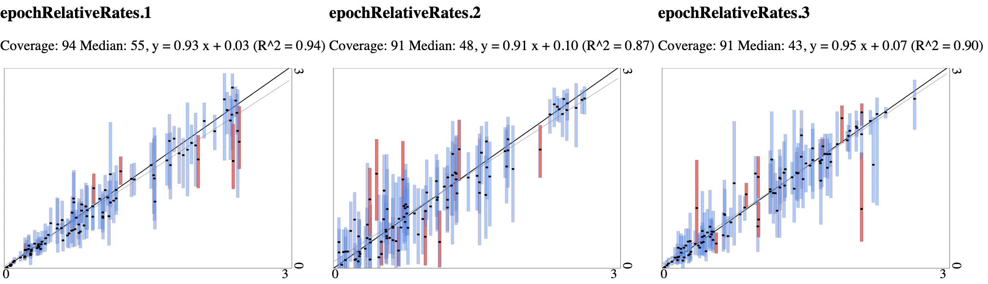
Since the x=y and regression lines match quite closely, we conclude that there appears to be good signal in the relative rates.
References
FK Mendes, R Bouckaert, LM Carvalho, AJ Drummond. How to validate a Bayesian evolutionary model. Systematic Biology, syae064, doi:10.1093/sysbio/syae064 2024